Triangulation for a better accuracy - Part 2

The first piece of this article discussed an overview of triangulation, how it works, its output and its benefits. So, let’s continue the discussion by explaining the triangulation types.

Triangulation can take several forms; data triangulation, methodological triangulation, theoretical triangulation, investigator triangulation and data analysis techniques triangulation.   

Data triangulation

This type involves using two or more data sources to study the phenomenon being researched. Basically, the information areas required for the research are the same but come from multiple sources. For example, collecting the primary and operational data to understand the reasons behind the declining sales 

Methodological triangulation

In this type, mixed methods are employed to study a unique phenomenon, including research and data collection methodologies. For instance, when quantitative and qualitative methods are used to study and understand the phenomenon.

Theoretical triangulation

When multiple theories and hypotheses are used to conduct the research, that’s called theoretical triangulation. For example, formulate different hypotheses to explain the reasons behind the declining sales. The churn-out rate last quarter increased due to a new tariff plan launched by the competitors, while our brand does not respond to this dynamic. This is one of the hypotheses. Another one can be: the bad quality of our network is the main reason; hence the research design can be developed taking into consideration these different hypotheses.             

Investigator triangulation

This type replies on the human for applying triangulation simply uses different researchers or data analysts in the study without prior discussion and collaboration between them. The idea is to remove the bias that might occur across the research process, whether in the designing or analysis stage.        

Data analysis triangulation 

In this type, a mix of data analysis techniques is applied in a study and conclude the outcome based on the output of these analysis techniques.

Triangulation in the research realm

To put theory into practice, I will demonstrate a case study from my previous work experience where data analysis triangulation has been employed. It was a concept design test. The study was about exploring the preference of several design concepts (3 design concepts). The three concepts are constructed in picture forms to be shown to the respondents. To achieve the objective effectively with high accuracy, a composite measure has been developed using latent and observed variables model. Preference Index (latent variable), the index comprises multiple observed variables (likability and purchase intention).

The observed variables have been measured using a ratio scale where respondents give their rating using a score from 0 to 100. A randomization plan is prepared to clear the order bias across the tested concepts. In the analysis stage, data analysis triangulation is employed using the following steps:

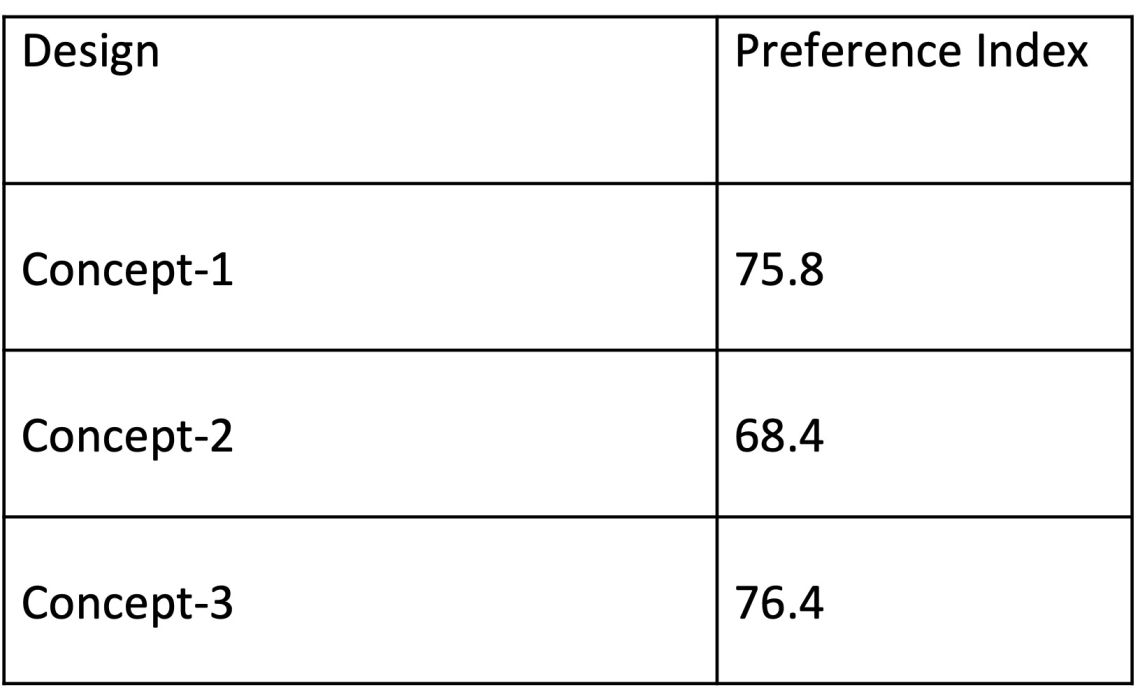
Firstly, descriptive analysis is done, and the mean score is calculated for all concepts for the observed variables. Preference index has calculated using a formula: Y = (ML + Mp)/ n

Where:

Y: preference index (index range is between 0 to 100, the higher, the better preference)

ML: mean score of likability.

Mp: mean score of purchase intention.

n: number of observed variables.

As shown in Table-1, it is very clear that concept-3 is the most preferred one. However, to increase confidence in the results and conclusion the second step is done.

Secondly, it has been planned to go beyond the stated responses by exploring the statistical probability of the preference. To estimate the probability of occurring, frequency distribution is done and picked up the highest score on the scale (Top Box: % of respondents rated the concept > 90 for each of the observed variables). Then, the probability of occurring (the probability of getting a rate > 90) has been estimated and using that probability of the observed variables to derive the preference index.

The process is a bit lengthy, but briefly; it is known that if the result follows the normal distribution shape, the probability of occurring can be estimated using the z-table. So, the steps are:

1. The scores (Top Box score) for the observed variables have been transformed to meet the normal distribution condition using the z-score formula.

2. Then looked up the corresponding probability of z-scores from the z- table.

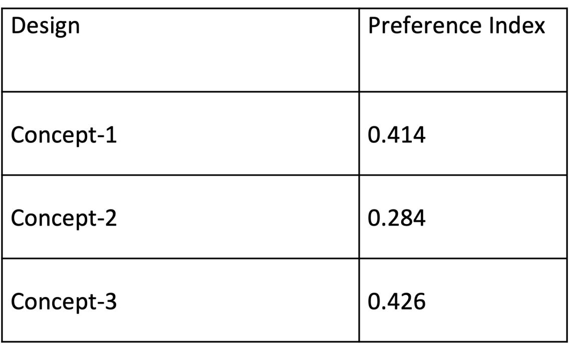
3. Finally, the index calculation is applied using this formula: Y = (PL + Pp)/ n

Where:

Y: preference index (index range is between 0 to 1, the higher, the better preference)

PL:: probability score of likability (likability rate is >90)

Pp: : probability score of purchase intention (purchase intention rate is >90)

n: : number of observed variables.

The results are summarised in Table-2. Looking at the index score, you can easily figure out that concept-3 is the most preferred one, followed by concept-1, and concept-2 comes at the third level. This is completely the same result that was reached in the first step (calculating the index based on the mean score). Therefore, the results from both analysis techniques converge, and now we are more confident about the conclusion.  

Triangulation return on investment

Although triangulation consumes effort and time, mainly in the execution stage, the comparison between the consumed resources and the obtained confidence level of the research results – that would not be reached with a single method – reveals a worthy return on investment, and it really helps for better accuracy. Let us triangulate then 😁.