Handling divergence in the results of mixed research methods

Research accuracy is important, and various methods are adopted to boost the accuracy level of the generated findings. Triangulation is one of the methods used to do this job. Triangulation is defined as the process of combining and integrating multiple approaches to increase the confidence of the generated research findings.

The core of triangulation is all about multiplicity; while having a single research phenomenon; multiple approaches are employed to study it. Hence it is all about mixed methods of employment. The figure below illustrates this mechanism. While we conduct a study to understand a unique phenomenon, it can be studied using multiple approaches e.g. quantitative and quantitative research or in another case utilizing more than one data source to reach the conclusion.

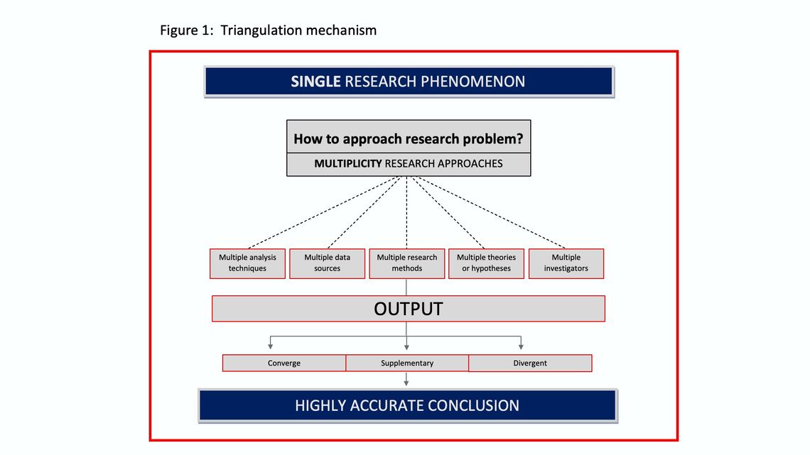
The process involves counterbalancing by taking the strength points of each approach while, at the same time, overcoming the weakness as the employed approaches complete each other, hence less error and higher accuracy can be maintained. For example, it is quite known that qualitative research has no capability of quantifying the research results (which quantitative research does), but it provides answers to why questions (which quantitative research does not). Triangulation allows both research tools to be employed and benefit from the strengths and overcome the weakness of each method. For more details on triangulation, please refer to this article .

As triangulation uses multiple approaches, does it mean the outcome is always different? And if it is different, is there a way to deal with such a situation? Well, the short answer for the first question is “No” and for the second one is “Yes”. Let’s elaborate more.                 

There are 3 expected outcomes of the triangulation which are converge, supplementary and divergent

1. Converge: the outcome of the different approaches is leading to the same conclusion. Here you would be quite confident about the research findings as the same conclusion has been confirmed through different methods.

2. Supplementary: the results of the approaches employed are not the same, but they explain and complete each other. In this case, you have a chance to complete the missing part of the story and fill in the blanks, so the conclusion is comprehensive.

3. Divergent: the results of the different approaches are shown different results and lead to divergent conclusions.

In the first two outcomes it is easy to draw the conclusion. But the situation gets harder with the divergent outcome as it becomes difficult to reach a conclusion with high confidence. So, what to do then?

A literature [a] review and textbooks on mixed research methods suggest four strategies can be used to handle the divergence of qualitative and quantitative research results: initiation, reconciliation, bracketing and exclusion.

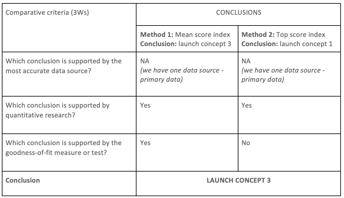
In addition to the strategies mentioned, I would like to suggest the Divergence Treatment Method (DTM) to reach a conclusion with confidence. The method relies on challenging the findings of the adopted analysis and approach through a comparison exercise based on three predefined comparative criteria (3Ws) illustrated in figure 2, with a goal of reaching the conclusion.

Before applying the method, it is recommended to ask a question: Is there any missing data that might change the diverging situation? If the answer is yes, go and collect it as it might lead to convergence or supplementary outcome, hence treating divergence would not be required. Otherwise, you have no option other than handling the divergence. 

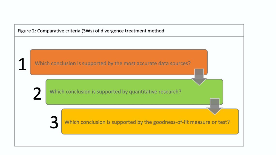
1. Which conclusion is supported by the most accurate data sources?

When multiple data types and sources are utilized, they are not always on the same level of accuracy, research design and limitations of each source have a direct impact on the finding's accuracy. With an assessment of each data source, the most accurate data source can be defined. For example, research based on samples is not the same as findings based on census for the same research problem. Both are different, yes, they are addressing the same research problem, but they are different in how to answer the research questions (research based on sample associated with a margin of error that leads to less accuracy compared to the research based on census) hence the accuracy varies. Another example is working on secondary data and primary data sources. The best practice is to assess the secondary data before using it in terms of different criteria: dependability, currency, design, objectives and errors. With the assessment you can understand the reliability level of the data. 

2. Which conclusion is supported by quantitative research?

If the mixed approaches consist of qualitative and quantitative research, the qualitative will not provide conclusive results, hence quantitative research findings are prioritized.

3. Which conclusion is supported by the goodness-of-fit measure or test?

Assessing the goodness-of-fit is common practice when applying the statistical analysis technique. The goodness-of-fit, the higher reliability and accuracy of results. If the research employs different analysis techniques, then drawing the conclusion can be done by examining the goodness-of-fit status of the analysis techniques. To do so correctly, the appropriate goodness-of-fit measure or test should be selected considering the required assumptions of each test. It is recommended to plan this in advance during the design and analysis stages of your project. To handle the divergence, two simple things need to be done.

Creating a convergence matrix

Simply, arrange the outcome of the divergence situation in a table, row side: comparative criteria, and column side: the conclusion of each method. Then, write the respective answer of each comparative criteria using the predefined choices: “Yes”, “No”, “Not Applicable - did not employ this”. The final output will look like the table below.

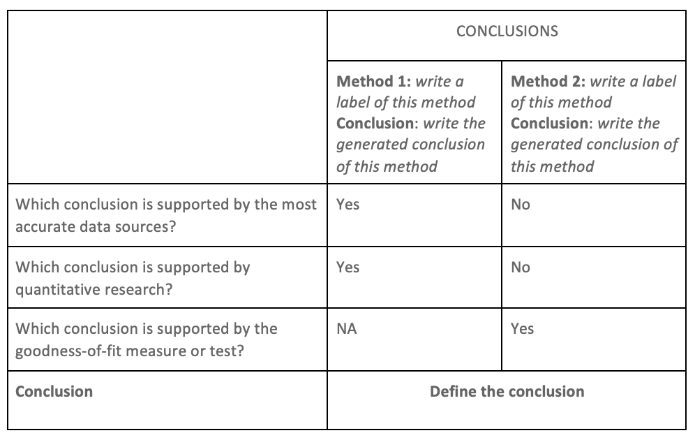
Now defining the conclusion is very easy, just look at the conclusion with more “yes”, which represents the conclusion.

To put theory into practice, let’s demonstrate a case study. The data is related to a concept testing study where the data analysis triangulation has been employed. The study was about exploring the preference of several concepts. The constructed concepts shown to the respondents then asked them to rate each one on several aspects. 

A composite measure has been developed using latent and observed variable model. Preference Index (latent variable) is derived from multiple observed variables (likeability and purchase intention).

The observed variables have been measured using ratio scale where respondents give their rating using a score from 0 to 100. A randomization plan was followed to control the extraneous variable which can occur from the selection bias (assigning a concept for testing) during the testing process. In the analysis stage, data analysis triangulation is employed using the following analysis techniques:

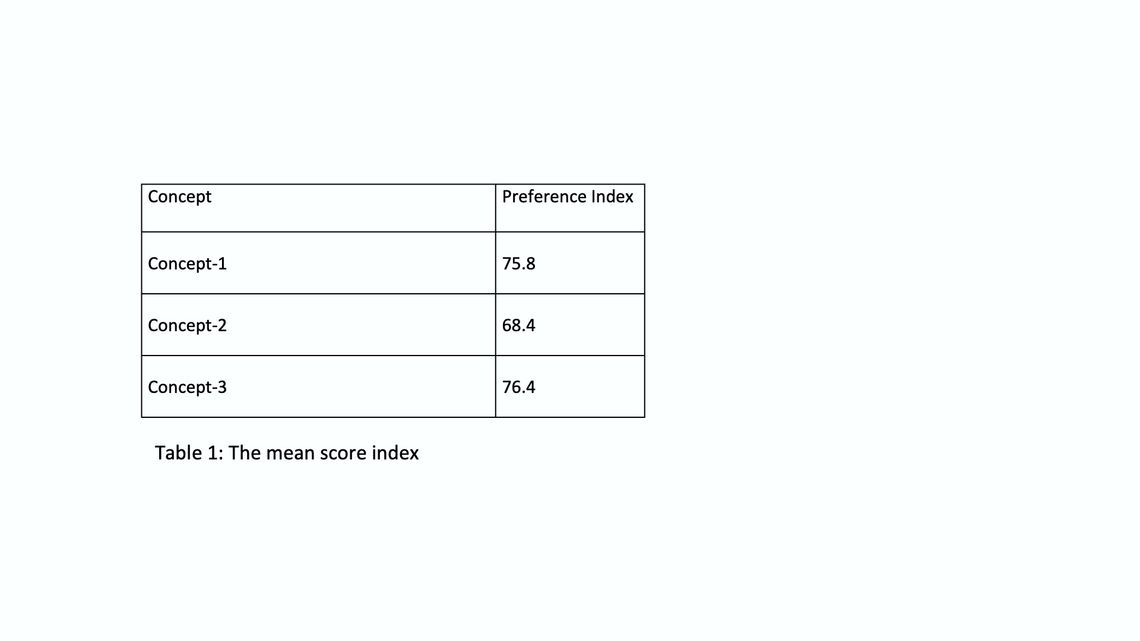
Mean score index

The descriptive analysis is done, and Mean score is calculated for the observed variables. Preference index has calculated using a formula: Y = (ML + Mp)/ n

Where:

Y: preference index (index range is between 0 to 100, the higher, the better preference)

ML: mean score of likability.

Mp: mean score of purchase intention.

n: number of observed variables.

As shown in Table (1), concept 3 is the most preferred one. However, to increase the confidence of results and conclusion the second step is conducted.

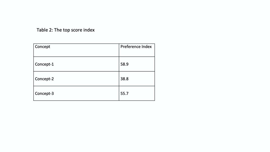
The top score index

The preference index has been calculated based on frequency distribution where the percentage of top rating score: % of respondents rated concept >= 80 for each of the observed variables is used to apply the index formula: Y = (TL + Tp)/ n

Where:

Y: preference index (index range is between 0 to 100, the higher, the better preference)

TL:: top rating score of likability (likability rated >=80)

Tp: : top rating score of purchase intention (purchase intention rated >=80)

n: : number of observed variables.

Table (2) summarizes the preference index based on the top rating score, and it indicates that concept 1 is the winner. This result is not aligned with the mean score index.

Now, we are facing a divergent outcome and want to know which conclusion has the highest confidence? To answer this, let us apply the divergence treatment method.

Creating convergence matrix

To complete the convergence matrix, it seems that we have the answer of all comparative criteria (3Ws) except the third one: Which conclusion is supported by the goodness-of-fit measure or test?

To examine the goodness-of-fit of each index, the following test and measure are done:

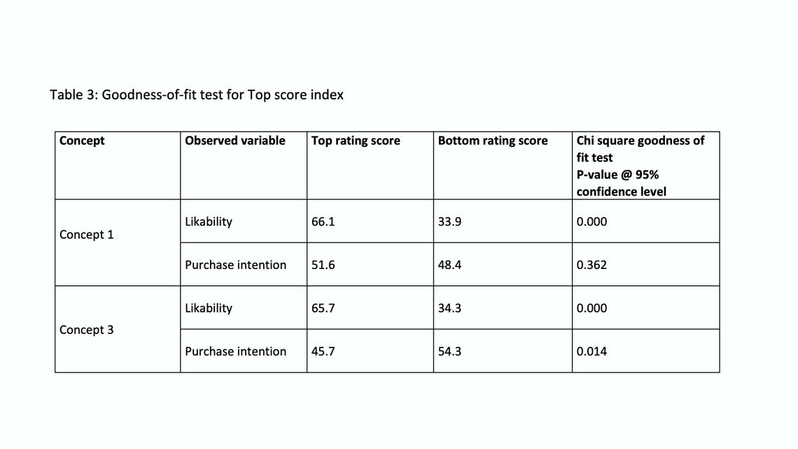
-        Chi-square goodness-of-fit test: It has been used to test the top score index (before running the test, the data has been transformed into categorical variable form, where the response of each observed variable is re-coded as 1 and 2. 1=top score rating is >= 80 and 2= bottom score rating is < 80 into new variables). This transformation has been made to meet the test assumptions, the rest of the assumptions have been considered as well (e.g. no cell has count of expected value less than 5). Given this situation, the Chi-square goodness-of-fit seems to be the suitable test.

             The null hypothesis: the frequencies of the observed variables are equal. 

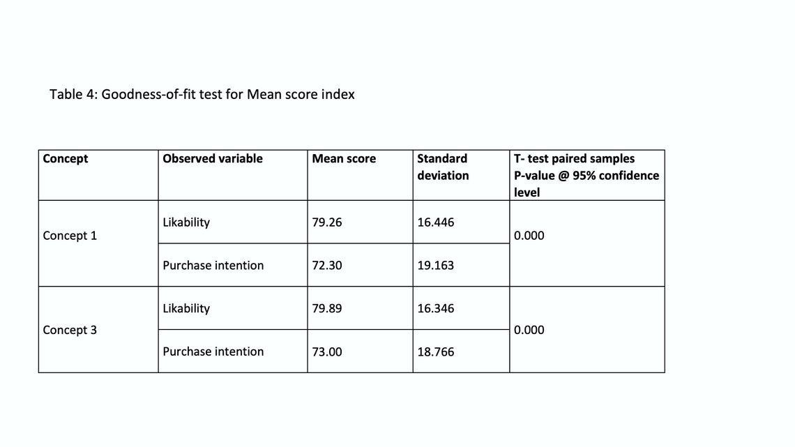
-        T test for paired samples: Given that the mean score index is derived from ratio data, t-test is an appropriate measure for the goodness-of-fit also the other assumptions (variables were almost normally distributed) are met as well.

              The null hypothesis: mean scores of the observed variables are equal. 

The summarized output of the goodness-of-fit tests are illustrated in table (3) and table (4) shown below. 

Top score index:

As shown in table (3), the chi-Square goodness-of-fit test indicates that the null hypothesis is true for purchase intention of concept 1, while it is rejected for other variables. Therefore, we conclude that the goodness-of-fit for this index partially exists as it does not fit the data for all components of the index across all concepts (observed variables). It is not a really good way to model the preference.  

Mean score index:

Looking at table (4), the test output explains that the null hypothesis is rejected for all concepts. Hence, the goodness-of-fit for this index completely exists since it does fit the data for all components of the index across all concepts (observed variables). In other words, it is more reliable to model the preference using this index.

Now, we are ready to create the convergence matrix and define the conclusion 

By the way, the standard deviation of the observed variables leads to the same conclusion. As lower standard deviation indicates higher goodness-of-fit is the winner.

Data-driven divergence treatment

As demonstrated in the case study, the divergence treatment method (DTM) considers an evidence-based tool of handling the divergence, it provides a data-driven decision of the conclusion. Yes, the method may end-up with ignoring a conclusion and overweight another, however what makes the researcher confident that the decision made based on data rather than a guess work. 

Reference

[a] Pluye, Pierre & Grad, Roland & Levine, Alissa & Nicolau, Belinda. (2014). Understanding divergence of quantitative and qualitative data (or results) In mixed methods studies. International Journal of Multiple Research Approaches. 3. 58-72. 10.5172/mra.455.3.1.58